Differentiable Wasserstein gradients

This notebook shows how to use oineus.diff and the visualization helpers together: compute a differentiable persistence diagram from a noisy point cloud, define losses against an ideal circle diagram, and plot diagram-space gradients from two Wasserstein-style objectives.

The point clouds are torch.Tensor objects throughout.

Setup

import math

import matplotlib.pyplot as plt
import torch

import oineus as oin
import oineus.diff as oin_diff

torch.set_default_dtype(torch.float64)

plt.rcParams.update({
    "figure.dpi": 120,
    "axes.spines.top": False,
    "axes.spines.right": False,
})

Clean and noisy samples

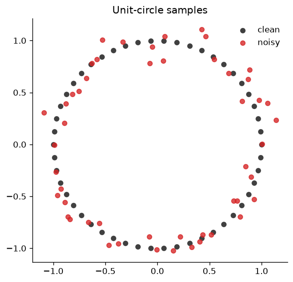
Start with 50 equally spaced points on the unit circle, then perturb the coordinates. The clean points define the target diagram; the noisy points are the variable we differentiate through.

n = 50
noise_scale = 0.08

angles = torch.arange(n) * (2.0 * math.pi / n)
clean_points = torch.stack((torch.cos(angles), torch.sin(angles)), dim=1)

torch.manual_seed(7)
noisy_points = (clean_points + noise_scale * torch.randn_like(clean_points)).clone()
noisy_points.requires_grad_(True)

clean_points.shape, noisy_points.shape, noisy_points.requires_grad

(torch.Size([50, 2]), torch.Size([50, 2]), True)

fig, ax = plt.subplots(figsize=(5, 5))
ax.scatter(clean_points[:, 0], clean_points[:, 1], s=30, label="clean", color="0.25")
ax.scatter(noisy_points.detach()[:, 0], noisy_points.detach()[:, 1], s=30, label="noisy", color="tab:red", alpha=0.8)
ax.set_aspect("equal", adjustable="box")
ax.set_title("Unit-circle samples")
ax.legend(frameon=False)
fig.tight_layout()

Differentiable H1 diagrams

We use a Vietoris-Rips filtration up to dimension 2 and extract the H1 diagram. The target diagram is detached because we want gradients only for the noisy diagram.

def h1_vr_diagram(points: torch.Tensor) -> torch.Tensor:
    fil = oin_diff.vr_filtration(points, max_dim=2, n_threads=4)
    dgms = oin_diff.persistence_diagram(
        fil,
        dualize=True,
        include_inf_points=False,
        n_threads=4,
    )
    return dgms[1]


clean_h1 = h1_vr_diagram(clean_points).detach()
noisy_h1 = h1_vr_diagram(noisy_points)
noisy_h1.retain_grad()


def diagram_bounds(*diagrams: torch.Tensor, pad_fraction: float = 0.12) -> dict[str, float]:
    pts = torch.cat([d.detach() for d in diagrams], dim=0)
    pts = pts[torch.isfinite(pts).all(dim=1)]
    lo = float(pts.min())
    hi = float(pts.max())
    span = max(hi - lo, 1.0)
    pad = pad_fraction * span
    return {"xmin": lo - pad, "xmax": hi + pad, "ymin": lo - pad, "ymax": hi + pad}


diagram_axis_bounds = diagram_bounds(clean_h1, noisy_h1)

clean_h1, noisy_h1

Error calling pthread_setaffinity_np: 22
Error calling pthread_setaffinity_np: 22
Error calling pthread_setaffinity_np: 22
Error calling pthread_setaffinity_np: 22

(tensor([[0.1256, 1.7526]]),
 tensor([[0.3595, 1.5784]], grad_fn=<_PDHelperBackward>))

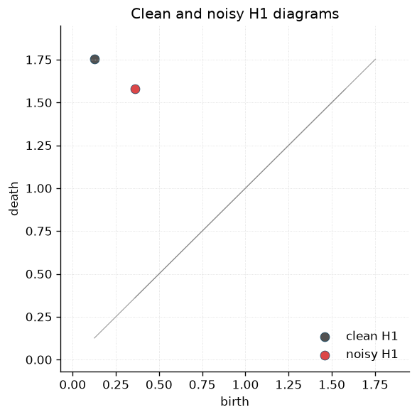
The clean and noisy diagrams each contain the dominant one-dimensional class from the sampled circle. Small perturbations move its birth and death coordinates.

fig, ax = plt.subplots(figsize=(5, 5))
oin.plot_diagram(
    {1: clean_h1.detach().cpu().numpy()},
    ax=ax,
    color={1: "0.2"},
    axis_bounds=diagram_axis_bounds,
    point_style={"s": 60},
    dim_label_fmt="clean H{dim}",
)
oin.plot_diagram(
    {1: noisy_h1.detach().cpu().numpy()},
    ax=ax,
    color={1: "tab:red"},
    axis_bounds=diagram_axis_bounds,
    point_style={"s": 60},
    dim_label_fmt="noisy H{dim}",
)
ax.set_title("Clean and noisy H1 diagrams")
ax.legend(frameon=False)
fig.tight_layout()

Wasserstein loss gradient

oineus.diff.wasserstein_cost uses the matching returned by Hera, then rebuilds the matched-pair cost in torch so autograd can differentiate it.

wasserstein_loss = oin_diff.wasserstein_cost(
    noisy_h1,
    clean_h1,
    wasserstein_q=2.0,
    wasserstein_delta=0.01,
    ignore_inf_points=True,
)
wasserstein_loss.backward(retain_graph=True)
wasserstein_grad = noisy_h1.grad.detach().clone()

wasserstein_loss.item(), wasserstein_grad

(0.0547285347071365, tensor([[0.4679, 0.0000]]))

Sliced Wasserstein loss gradient

Now clear the retained diagram gradient and differentiate the sliced Wasserstein loss on the same noisy diagram. We fix the torch seed so the random projection directions are reproducible.

noisy_h1.grad = None
noisy_points.grad = None

torch.manual_seed(11)
sliced_loss = oin_diff.sliced_wasserstein_distance(
    noisy_h1,
    clean_h1,
    n_directions=256,
    ignore_inf_points=True,
)
sliced_loss.backward()
sliced_grad = noisy_h1.grad.detach().clone()

sliced_loss.item(), sliced_grad

(0.22522903087243942, tensor([[ 0.9414, -0.0189]]))

Overlay the two gradients

Both fields are drawn on the noisy H1 diagram. The first call plots the noisy diagram points; the second call reuses the same axes and sets plot_points=False, so only the second arrow layer is added. The arrows below use descent=True, so they show the negative gradient direction used by a minimizer.

fig, ax = plt.subplots(figsize=(6, 6))

oin.plot_diagram_gradient(
    {1: noisy_h1.detach()},
    {1: wasserstein_grad},
    ax=ax,
    descent=True,
    plot_points=True,
    axis_bounds=diagram_axis_bounds,
    title="H1 descent directions on the noisy diagram",
    diagram_color="0.25",
    point_style={"s": 70, "alpha": 0.65},
    quiver_style={
        "color": "tab:blue",
        "alpha": 0.85,
        "width": 0.006,
        "scale_units": "xy",
        "scale": 4.0,
        "angles": "xy",
        "label": "Wasserstein descent",
    },
)

oin.plot_diagram_gradient(
    {1: noisy_h1.detach()},
    {1: sliced_grad},
    ax=ax,
    descent=True,
    plot_points=False,
    quiver_style={
        "color": "tab:orange",
        "alpha": 0.9,
        "width": 0.004,
        "scale_units": "xy",
        "scale": 4.0,
        "angles": "xy",
        "label": "sliced Wasserstein descent",
    },
)

ax.scatter(
    clean_h1[:, 0],
    clean_h1[:, 1],
    s=90,
    facecolors="none",
    edgecolors="black",
    linewidths=1.4,
    label="clean H1 target",
)
ax.legend(frameon=False, loc="upper left")
ax.set_aspect("equal", adjustable="datalim")
fig.tight_layout()

Ignoring fixed y limits to fulfill fixed data aspect with adjustable data limits.

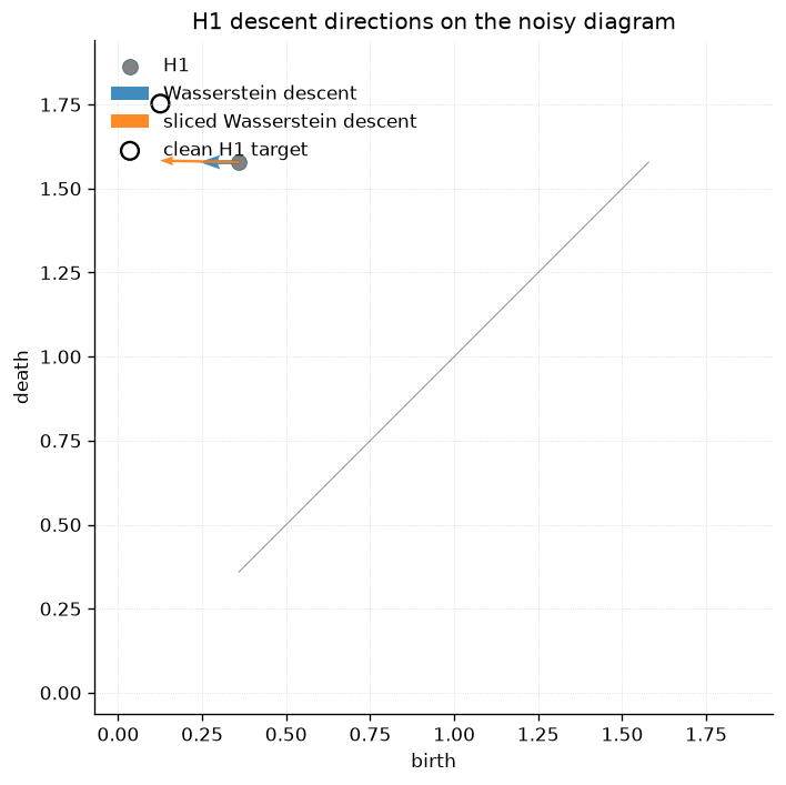
The matching-based and sliced losses can point in different diagram-space directions even when they compare the same two diagrams. In a full optimization loop, those diagram gradients continue backward through the VR filtration to noisy_points.grad.